Gene Set Enrichment Analysis

Introduction

categoryCompare2 was originally designed to work with enrichments generated via hypergeometric enrichment, or over-representation. However, there are some limitations to that method, some of which can possibly be overcome using gene-set enrichment analysis, or GSEA. This vignette shows how to use categoryCompare2 to work with GSEA enrichments.

Sample Data

To make the concept more concrete, we will examine data from the microarray data set estrogen available from Bioconductor. This data set contains 8 samples, with 2 levels of estrogen therapy (present vs absent), and two time points (10 and 48 hours). A pre-processed version of the data is available with this package, the commands used to generate it are below. Note: the preprocessed one keeps only the top 100 genes, if you use it the results will be slightly different than those shown in the vignette.

library("affy")
library("hgu95av2.db")
library("genefilter")
library("estrogen")
library("limma")
library("categoryCompare2")
library("GO.db")
library("org.Hs.eg.db")

datadir <- system.file("extdata", package = "estrogen")
pd <- read.AnnotatedDataFrame(file.path(datadir,"estrogen.txt"), 
    header = TRUE, sep = "", row.names = 1)
pData(pd)

##              estrogen time.h
## low10-1.cel    absent     10
## low10-2.cel    absent     10
## high10-1.cel  present     10
## high10-2.cel  present     10
## low48-1.cel    absent     48
## low48-2.cel    absent     48
## high48-1.cel  present     48
## high48-2.cel  present     48

Here you can see the descriptions for each of the arrays. First, we will read in the cel files, and then normalize the data using RMA.

currDir <- getwd()
setwd(datadir)
a <- ReadAffy(filenames=rownames(pData(pd)), phenoData = pd, verbose = TRUE)

## 1 reading low10-1.cel ...instantiating an AffyBatch (intensity a 409600x8 matrix)...done.
## Reading in : low10-1.cel
## Reading in : low10-2.cel
## Reading in : high10-1.cel
## Reading in : high10-2.cel
## Reading in : low48-1.cel
## Reading in : low48-2.cel
## Reading in : high48-1.cel
## Reading in : high48-2.cel

setwd(currDir)

eData <- affy::rma(a)

## Warning: replacing previous import 'AnnotationDbi::tail' by 'utils::tail' when
## loading 'hgu95av2cdf'

## Warning: replacing previous import 'AnnotationDbi::head' by 'utils::head' when
## loading 'hgu95av2cdf'

## Background correcting
## Normalizing
## Calculating Expression

To make it easier to conceptualize, we will split the data up into two eSet objects by time, and perform all of the manipulations for calculating significantly differentially expressed genes on each eSet object.

So for the 10 hour samples:

e10 <- eData[, eData$time.h == 10]
e10 <- nsFilter(e10, remove.dupEntrez=TRUE, var.filter=FALSE, 
        feature.exclude="^AFFX")$eset

e10$estrogen <- factor(e10$estrogen)
d10 <- model.matrix(~0 + e10$estrogen)
colnames(d10) <- unique(e10$estrogen)
fit10 <- lmFit(e10, d10)
c10 <- makeContrasts(present - absent, levels=d10)
fit10_2 <- contrasts.fit(fit10, c10)
eB10 <- eBayes(fit10_2)
table10 <- topTable(eB10, number=nrow(e10), p.value=1, adjust.method="BH")
table10$Entrez <- unlist(mget(rownames(table10), hgu95av2ENTREZID, ifnotfound=NA))

And the 48 hour samples we do the same thing:

e48 <- eData[, eData$time.h == 48]
e48 <- nsFilter(e48, remove.dupEntrez=TRUE, var.filter=FALSE, 
        feature.exclude="^AFFX" )$eset

e48$estrogen <- factor(e48$estrogen)
d48 <- model.matrix(~0 + e48$estrogen)
colnames(d48) <- unique(e48$estrogen)
fit48 <- lmFit(e48, d48)
c48 <- makeContrasts(present - absent, levels=d48)
fit48_2 <- contrasts.fit(fit48, c48)
eB48 <- eBayes(fit48_2)
table48 <- topTable(eB48, number=nrow(e48), p.value=1, adjust.method="BH")
table48$Entrez <- unlist(mget(rownames(table48), hgu95av2ENTREZID, ifnotfound=NA))

And grab all the genes on the array to have a background set.

For both time points we have generated a list of genes that are differentially expressed in the present vs absent samples.

We will calculate GSEA enrichments using fgsea, and then compare the enrichments between the two timepoints.

Create Annotations and Enrich

bp_annotation = get_db_annotation("org.Hs.eg.db", features = table10$Entrez, annotation_type = "BP")

g10_ranks = table10$logFC
names(g10_ranks) = table10$Entrez
g10_features = new("gsea_features", ranks = g10_ranks, annotation = bp_annotation)
g10_enrich = gsea_feature_enrichment(g10_features, min_features = 20,
                                     max_features = 200)

g48_ranks = table48$logFC
names(g48_ranks) = table48$Entrez
g48_features = new("gsea_features", ranks = g48_ranks, annotation = bp_annotation)
g48_enrich = gsea_feature_enrichment(g48_features, min_features = 20,
                                     max_features = 200)

Combine and Find Significant

bp_combined <- combine_enrichments(g10 = g10_enrich,
                                  g48 = g48_enrich)

bp_sig <- get_significant_annotations(bp_combined, padjust <= 0.001)
bp_sig@statistics@significant

## Signficance Cutoffs:
##   padjust <= 0.001
## 
## Counts:
##    g10 g48 counts
## G1   1   1     96
## G2   1   0     19
## G3   0   1     99
## G4   0   0   2953

Generate Graph

bp_graph <- generate_annotation_graph(bp_sig)
bp_graph

## A cc_graph with
## Number of Nodes = 214 
## Number of Edges = 12659 
##    g10 g48 counts
## G1   1   1     96
## G2   1   0     19
## G3   0   1     99

bp_graph <- remove_edges(bp_graph, 0.8)

## Removed 12380 edges from graph

bp_graph

## A cc_graph with
## Number of Nodes = 214 
## Number of Edges = 279 
##    g10 g48 counts
## G1   1   1     96
## G2   1   0     19
## G3   0   1     99

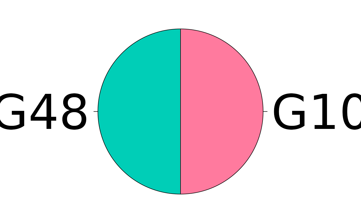
bp_assign <- annotation_combinations(bp_graph)
bp_assign <- assign_colors(bp_assign)

Find Communities

It is useful to define the annotations in terms of their communities. To do this we run methods that find and then label the communities, before generating the visualization and table.

bp_communities <- assign_communities(bp_graph)
bp_comm_labels <- label_communities(bp_communities, bp_annotation)

Visualize It

bp_network <- graph_to_visnetwork(bp_graph, bp_assign, bp_comm_labels)

vis_visnetwork(bp_network)

Robert M Flight